Denoising data using MAGIC

What is dropout?

One of the primary drawbacks of scRNA-seq is that current methods only capture 10-40% of mRNA present in each cell [1, 2, 3, 4]. As a result, all genes in all cells are undercounted, and lowly expressed genes may be recorded at 0s in the gene expression matrix despite being expressed. This undercounting of mRNA molecules in single cells is called dropout.

Dropout is an issue because we might often about expression of those genes (e.g. transcription factors that mark a specific cell type). Beyond marker genes, we also care about how sets of genes are expressed together (or not) across many cells. This information can be used to learn gene-gene relationships and putative regulatory interactions between genes.

Simulating

To demonstrate this, let’s get creative. It’s hard to establish a “ground truth” for single cell data, so we picked a large bulk C. elegans time course and simulated a 20% mRNA capture efficiency by down-sampling molecules in the dataset. On the left is the original data for 9861 genes in 206 worms, and the right is the simulated undercounted data.

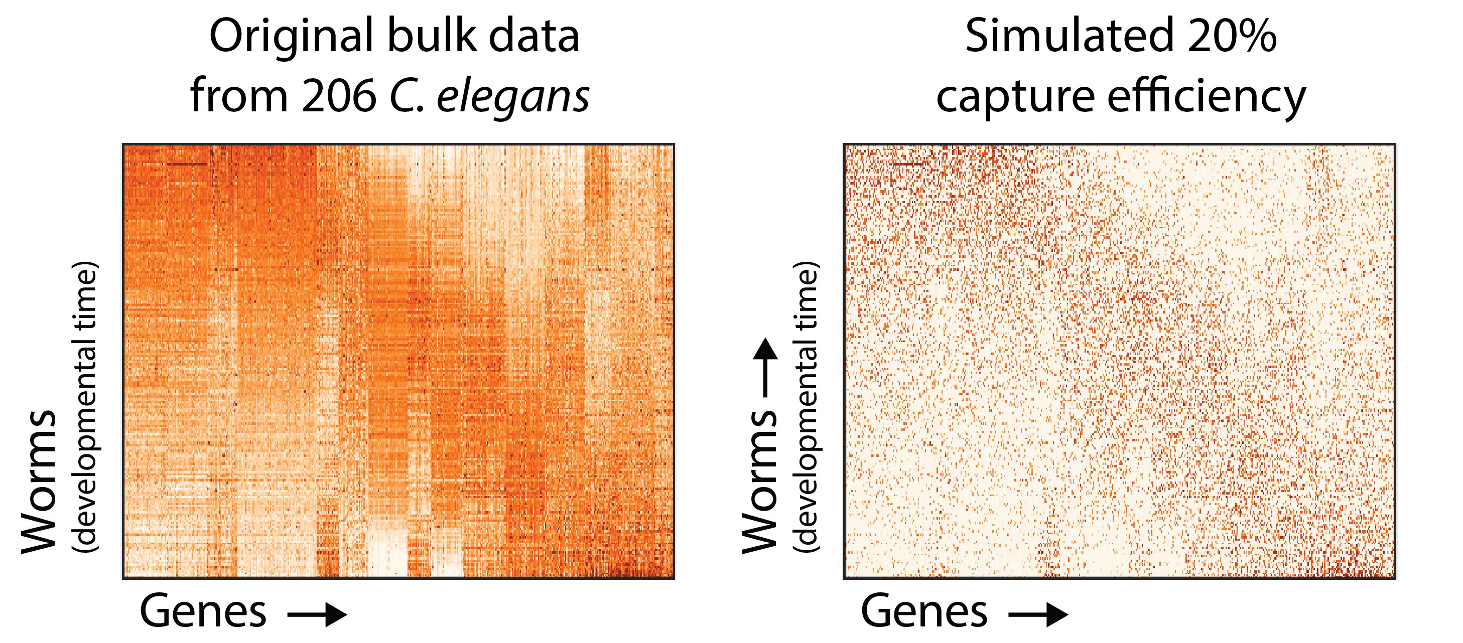
You can see here how the number of zero values in the matrix is increased by simulating an 80% capture rate per cell (i.e. the probability of detecting a each molecule of each mRNA is 20%). To understand how badly this can obscure the dynamics of gene expression genes, consider the following plots.

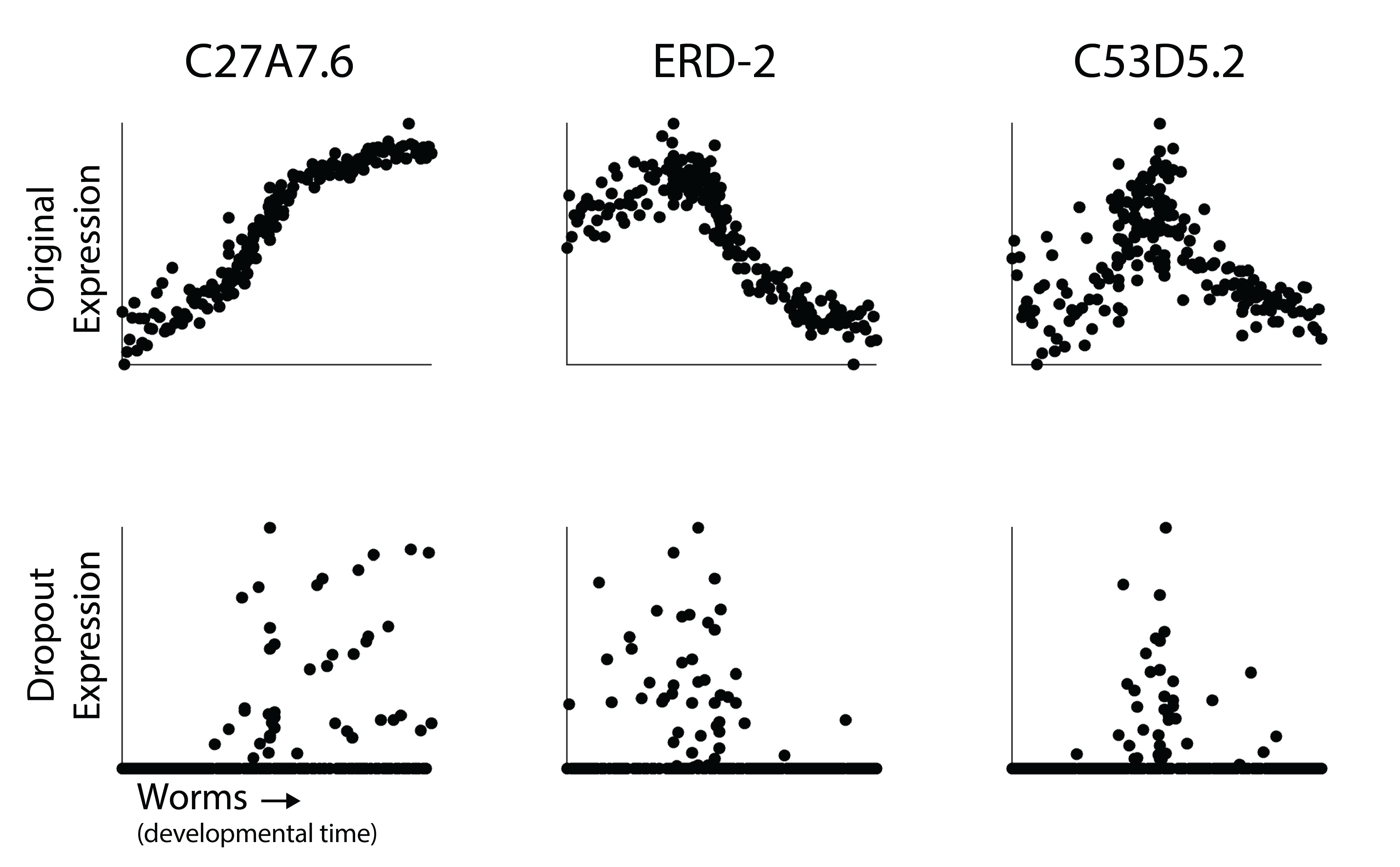
In each scatterplot, each dot is an expression profile. The y-axis is expression level of that gene either in the raw time course (top) or after simulated dropout (bottom). The bulk samples are arranged on the x-axis in the ordering of the time course. You can think of this as a small single cell experiment where we’ve identified an axis of pseudotime that orders cells along a developmental trajectory.

Although the dynamics in expression are clear in the raw time course, I would be hard pressed to describe how they change over time after dropout. So how do we recover those dynamics? Are we just unable to characterize gene expression changes at resolution in single cell RNA-seq?

Of course not!

Using redundancy to denoise gene expression

We can impute or denoise gene expression data because of two forms of redundancy.

First, the cells are redundant. In a dataset there many be dozens, hundreds, or thousands of the same cell type. Even if we miss expression of a given marker gene in one cell of the same type, if we see it in all the other cells of that type, then we can guess that it’s probably expressed in that cell. In this developmental time course, even if we miss measuring expression of Gene A at time t, if we see it at time t-1 and time t+1, then it’s probably expressed at time t.

The second factor working in our favor is that the expression of each gene is not completely independent of other genes in the matrix. Because multiple genes can be co-regulated in the same gene module, we can use information about the expression of some of the genes to infer the expression the others. For example, imagine that when a given transcription factor is expressed, 10 other genes are upregulated. Knowing this, we can infer from the fact that 8 of them are expressed, that the other 3 genes in the module are likely expressed too.

So how do we take advantage of these facts? We can’t easily encode information about gene modules or cell types, so we need to simultaneously learn those relationships and correct them. That’s not easy. There are a number of compelling algorithms for solving this problem when the missing values are known (i.e. you only want to correct zero entries). This formulation is also called the Netfix Problem or matrix completion and is discussed in the previous section.

However, we don’t even know which genes are true zero (i.e. not expressed) and which are biological zeroes (i.e. not expressed). Even further, its not just lowly expressed genes that are affected by dropout, but all mRNA molecules that are undersampled. This means we also would like to remove noise from expression of all genes. So we need to take a different approach.

Using MAGIC to denoise gene expression

To recover these relationships, we developed MAGIC (van Dijk, D. et al. 2018.). MAGIC first learns the underlying structure, or manifold, of the data, and then smooths gene expression values over this manifold. To do this, MAGIC uses a cell-cell affinity graph to construct a Markov diffusion operator that is then used to diffuse data between cells, in the process filling in missing values and generally denoising the data.

Now reading that last sentence, there’s a pretty high chance you thought something along the lines of, “Uses a diffusion what…?” Dont worry. Intuitively, you can think of this as saying “If Cell A and Cell B share expression levels of 99% of their genes, and Cell A expresses Gene X, then Cell B probably expresses Gene X at roughly the same level”. If you want to learn more, We wrote a whole blog post about the MAGIC algorithm.

Here, our goal is to demonstrate that MAGIC works and how to use it in a single cell workflow. First, let’s revisit those three genes from the worm datasets above.

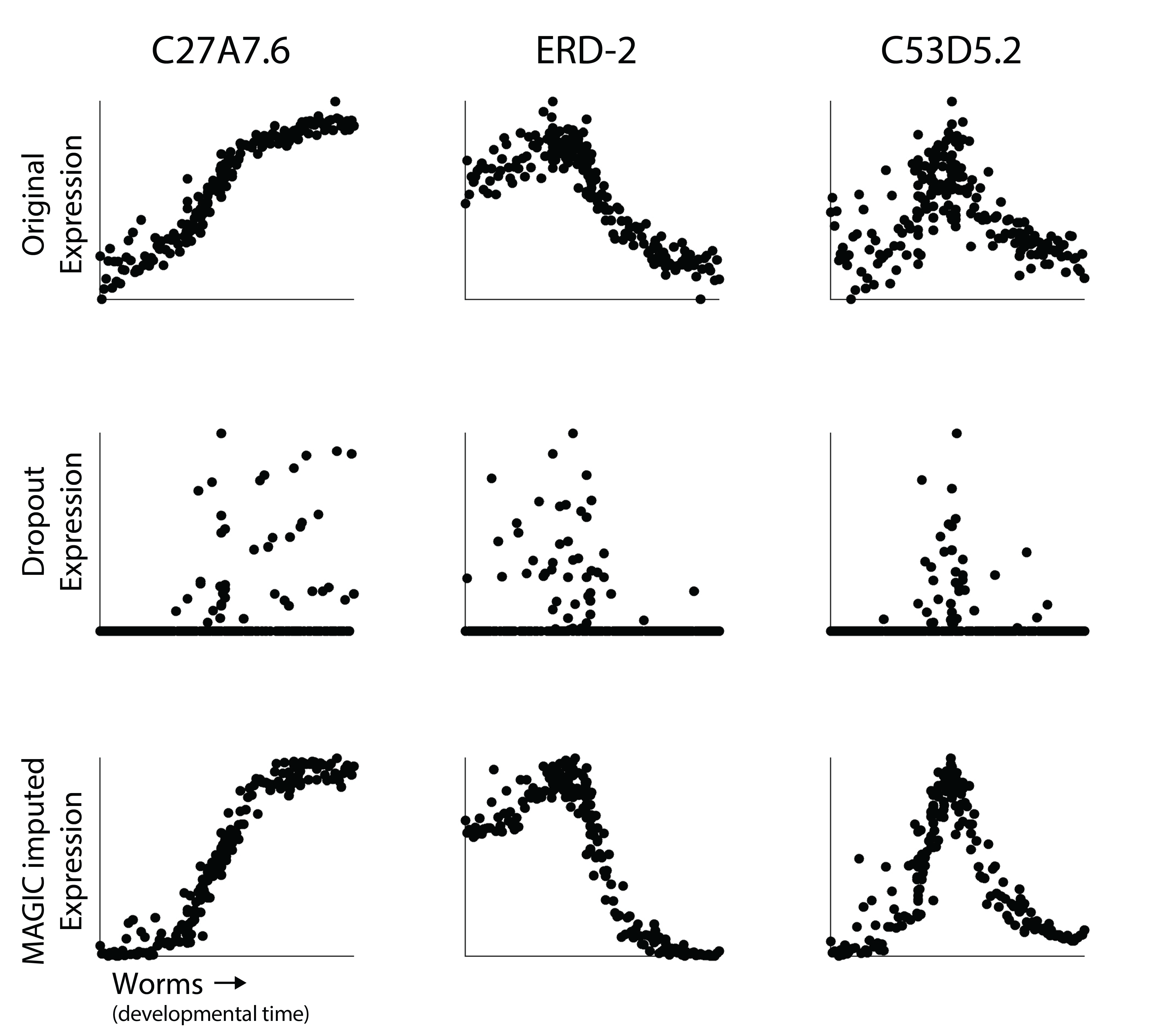
It should be fairly clear here that using MAGIC reveals the non-linear dynamics of expression of each gene over time. Now you may notice that the imputed gene expression values are a bit smoother than the original data. The is especially clear for C53D5.2. In MAGIC, our goal is to smooth gene expression values. What happens is that we don’t only remove variation due to undersampling, but we also remove noise associated with some of the biological heterogeneity in the dataset. As we will discuss in the next section, the amount of smoothing can be user-adjusted (although the MAGIC software tries to identify an optimal t).

Now let’s return to the full gene expression matrix.

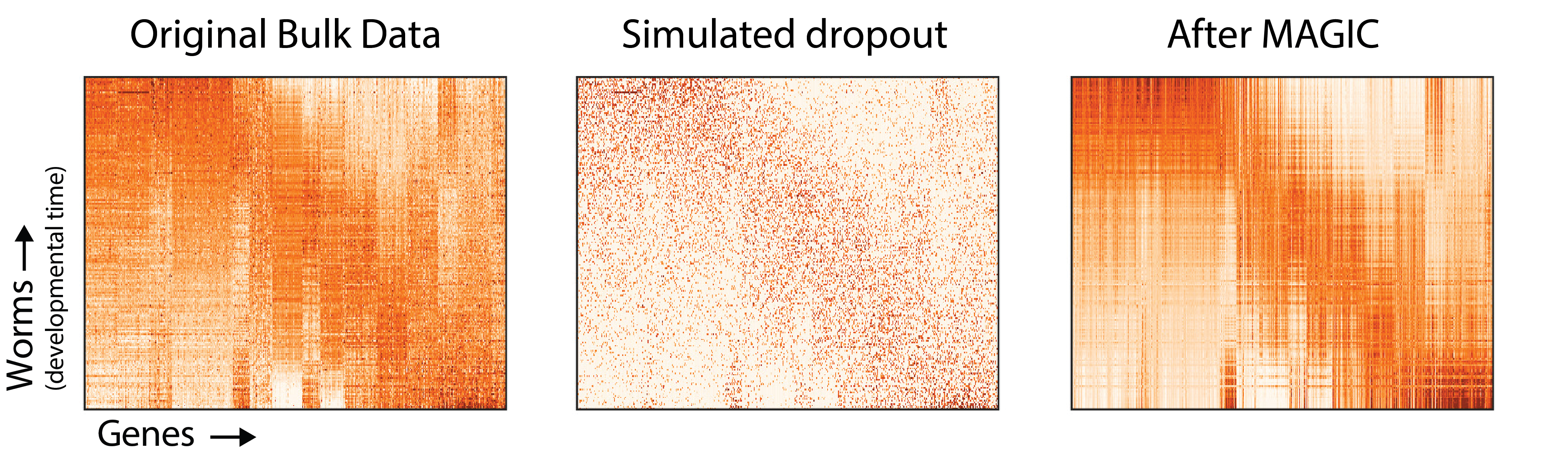
Again, it’s clear that MAGIC recovers the underlying structure of the original gene expression matrix, and removes biological noise. Although we can’t perfectly recreate the original gene expression matrix (and may not want to), the gene expression matrix after MAGIC is much closer to the original than the dataset with simulated dropout.

Using MAGIC on single cell data

Now that we’ve seen how MAGIC works, let’s go over how to use MAGIC for analysis of single cell data. MAGIC is implemented in Python. The source code is available on GitHub: https://www.github.com/KrishnaswamyLab/MAGIC with documentation on ReadTheDocs: https://magic.readthedocs.io/en/stable/.

Installing MAGIC is easy:

$ pip install --user magic-impute

and applying it to single cell data doesn’t take much work either

import magic

magic_operator = magic.MAGIC()
data_magic = magic_operator.fit_transform(data_sq)

Now it’s important to note that although you can easily run MAGIC using default parameters, MAGIC builds a cell similarity graph from the data to do imputation. The way you build this graph can have profound impact on the results on the output. We discuss graphs more thoroughly in visualizing data using PHATE, but the essential thing to know is that a graph represents information about which cells are close to each other. If you build a graph that connects cells that shouldn’t be connected, then imputation won’t work properly.

To quickly see the effect of imputation, let’s examine expression of two genes in a dataset of T cell activation from Datlinger et al., (2017). Here, Jurkat T cells were stimulated with anti-CD3/CD28 beads followed by scRNA-seq.

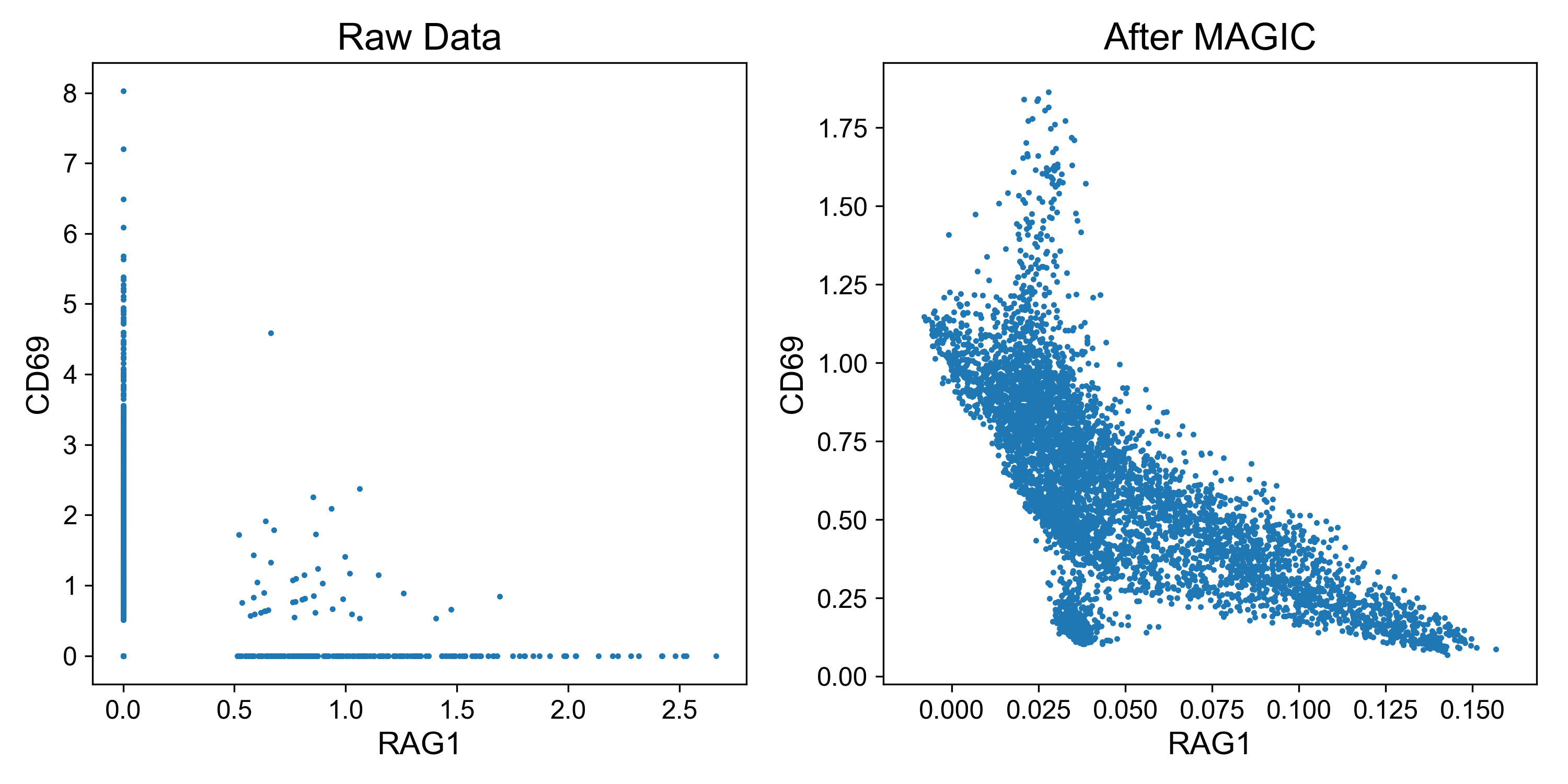
CD69 is a classic marker of T cell activation and is upregulated shortly after activation (Ziegler et al. 1994). RAG1 is a recombinase important for thymocyte differentiation and is downregulated after TCR stimulation (Turka et al. 1991). Thus, it is expected that expression of these genes should be inversely related.

Examining expression of the raw data, it’s difficult to observe this relationship because so many read counts are 0. However, on the right it’s clear that cells with highest expression of CD69 (i.e. activated cells) have lowest expression of RAG1 and visa versa.

When to use MAGIC

I will run MAGIC on almost every dataset I work with, but I don’t use it in all analysis. One major application where I use raw data is in differential expression analysis, especially between subpopulations of cells. This is because MAGIC tends to smooth out differences between closely related cells and would risk removing relevant signal.

FAQ: