If you understand the phrase “eigendecomposition of a graph Laplacian”, you can skip to the next section. Otherwise, I highly recommend you read on.
Wait, no one said there would be math
I imagine that some of you might be looking at the header of this section and feel slightly betrayed. You might be thinking, “I thought I was done with algebra!” Now it’s true that many people can do single cell analysis without having a grasp of the concepts we’re going to cover in this section. However, as my mom always told me growing up, just because you can, doesn’t mean you should.
Almost all of the packages that you’ll encounter while doing single cell analysis abstract away the math behind shiny APIs and wrappers. One of the issues here is that although you may understand the concept of something like library size normalization, you probably don’t realize the implications this has on things like calculating the distance between cells or estimating expression of a gene in a population.
Single cell analysis is full of choices: Should I use Euclidean or Cosine distances as my distance function? What perplexity should I pass to t-SNE? How many neighbors should I use when building a kNN graph? Should I use a negative binomial or zero-inflated model when calculating differential expression? You may have heard of some of these terms, but getting the most out of single cell data requires a baseline knowledge of how these methods work.
Objectives
We’re not going to spend too much time here going through the nitty gritty of matrices and graphs that you’d get in a set of serious math textbooks. The goal of this section is to help you enough familiarity of vectors and graphs to the point where you can understand the difference between PHATE and t-SNE on an algorithmic level.
We’re going to start by talking about high dimensional vectors and matrices, then discuss distance functions. We’ll move on to graphs and matrix representations of graphs such as the weight matrix. Finally, were going to discuss eigenvectors and discuss how they underly algorithms like PCA.
Vectors
What’s a vector, Victor?
That clip above is from the 1980 film Airplane!. Now you might be as confused as Peter Graves when you hear my talking about vectors, but don’t worry; they’re not so complicated.
Well actually, they are. I used to hate when people said, “This sounds complicated, but it’s actually simple.” Some of the math we go through here is going to be very complicated, and you shouldn’t feel bad if you don’t understand on the first go. Focus on the high level interpretation at first, and the nuances will come as you gain experience and experiment.
But really, what’s a vector?
In physics, you probably learned the term vector in the context of scalar. The typical definition here goes something like “a scalar is a quantity associated with a magnitude and a vector is a quantity associated with a magnitude and a direction”. Although scalars and vectors are important concepts, I don’t like this definition. I think it’s overly confusing and mixes up some of the nice properties of numbers.
Instead, lets start with real numbers. Real numbers are numbers without a complex component (i.e. the numbers we’re used to dealing with every day). $1$ is a real number. So is $\pi$ and Avagadro’s number $10^{23}$.
The next important concept is the real coordinate space, sometimes called Euclidean space or Cartesian space (Wolfram). These n-dimensional coordinate spaces are often denoted as $\mathbb{R} ^n$. To get a sense for real coordinate space, let’s consider a simple 2-dimensional vector, $\mathbf{a}$ (i.e. a real number in $\mathbb{R}^2$).
$$\mathbf{a} = \begin{bmatrix}x_1\\x_2\end{bmatrix}$$
This probably isn’t very clear. Here, $\mathbf{a}$ is a vector in $\mathbb{R} ^2$. $x_1$ is the value of $\mathbf{a}$ in the first dimension of $\mathbb{R} ^2$ and $x_2$ is the value of $\mathbf{a}$ in the second dimension of $\mathbb{R}^2$. Although $\mathbf{a}$ is technically a vector in $\mathbb{R}^2$, we haven’t actually specified which vector it is. Let’s pick one.
$$\mathbf{a} = \begin{bmatrix}1\\2\end{bmatrix}$$
Here we have it, a real live vector! So… what does this mean? To help understand, let’s create a in Python. The Python package NumPy is the fundamental package for scientific and numerical computing in Python. The core of numpy is the n-dimensional array (ndarray). It couldn’t be simpler for us to create $\mathbf{a}$ using numpy.
>>> import numpy as np
>>> a = np.array([1,2])
>>> a
array([1, 2])
Numpy uses the array class to represent vectors of any length. We can plot this vector using matplotlib.
import matplotlib.pyplot as plt

fig, ax = plt.subplots(1, figsize=(5.1,5))

xlim = (-.1,3)
ylim = (-.1,3)

ax.scatter(x[0], x[1], s=75)

ax.set_xlim(xlim)
ax.set_ylim(ylim)

ax.set_xticks(np.arange(0, xlim[1] + 1))
ax.set_yticks(np.arange(0, ylim[1] + 1))

ax.set_xlabel(r'$x_{1}$',fontsize=20)
ax.set_ylabel(r'$x_{2}$',fontsize=20,rotation=0)

ax.text(1,1.7, '[1,2]')

fig.tight_layout()
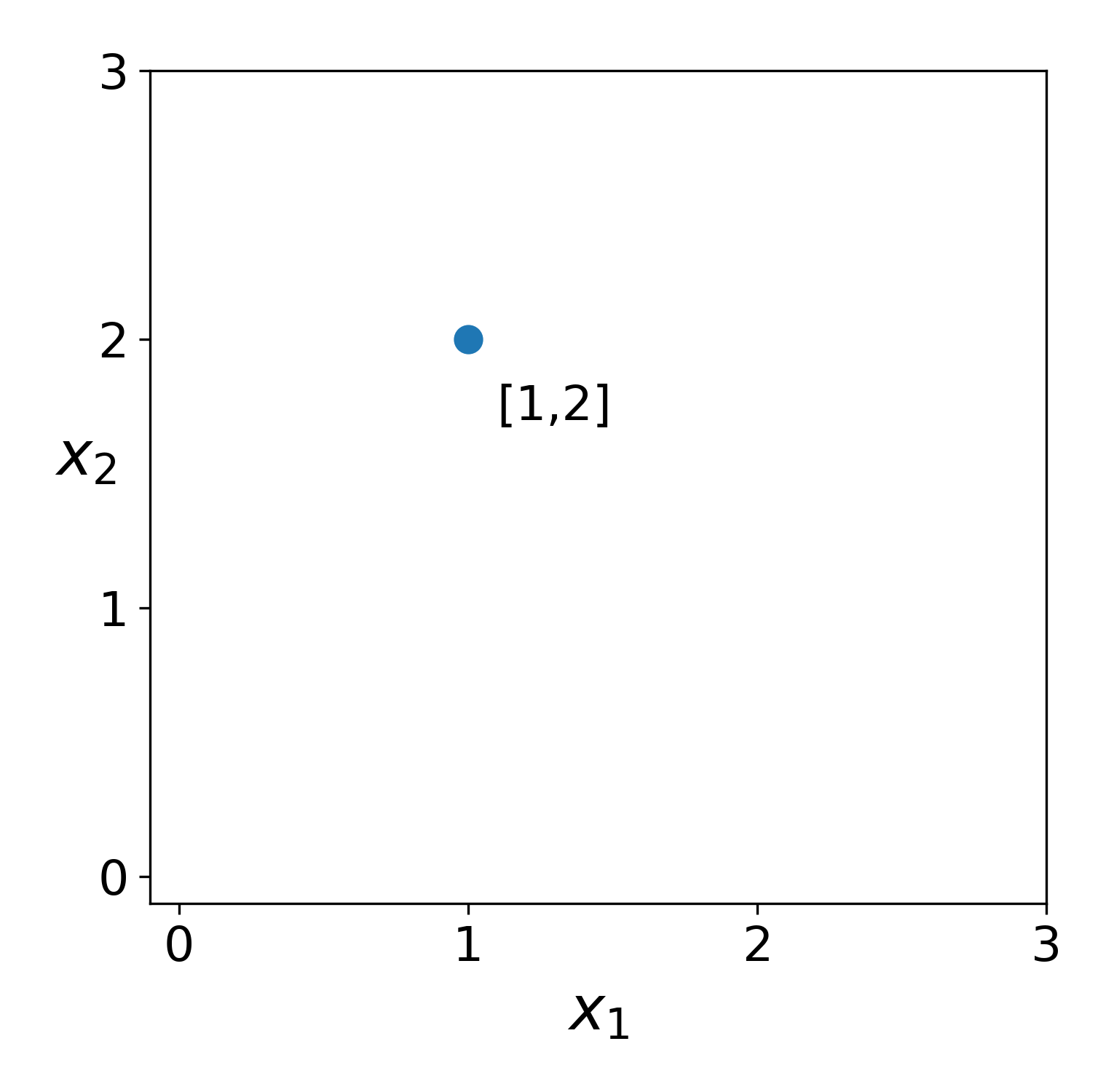
Here, we’re looking at $\mathbf{a}$ plotted in two dimensions, i.e. $\mathbb{R}^2$. When drawn this way, $\mathbf{a}$ looks like a point. You might be thinking “What’s the direction of $\mathbf{a}$?” My suggestion is to just forget about the concept of direction. A vector is a real number with quantities defined in a real coordinate space $\mathbb{R}^n$. With this definition, a scalar is simply a vector in $\mathbb{R}^1$. I think this is a much more intuitive way to think about vectors for our purposes.
What do vectors have to do with single cells?
In short, the reason we need to understand vectors is because in single cell datasets, we’re going to be analyzing cells as vectors in a real coordinate space $\mathbb{R}^m$ where $m$ is the number of genes in the genome of the organism from which the cell originated. In the previous section, we discussed a vector $\mathbf{a}$ in $\mathbb{R}^2$. However, vectors can exist in any number of dimensions.
Let’s define a new vector, $\mathbf{a_2}$ in $\mathbb{R}^3$.
$$\mathbf{a} = \begin{bmatrix}x_1=2\\x_2=4\\x_3=1\end{bmatrix}$$
We can just as easily create $\mathbf{a}$ in numpy and plot it to see what it looks like.
import numpy as np
a2 = np.array([1,2])
a2
array(2, 4, 1])
And using some tricks with matplotlib, we can plot it.
import matplotlib.pyplot as plt
from mpl_toolkits.mplot3d import Axes3D
fig = plt.figure()
fig.set_size_inches(6,5)
ax = fig.add_subplot(111, projection='3d')

xlim = (0,5)
ylim = (0,5)
zlim = (0,5)
ax.scatter(a2[0], a2[1], a2[2], s=75)

ax.plot([2,2], [4,4], [0,1], c='k')

ax.set_xlim(xlim)
ax.set_ylim(ylim)
ax.set_zlim(zlim)

ax.set_xticks(np.arange(xlim[0], xlim[1] + 1))
ax.set_yticks(np.arange(ylim[0], ylim[1] + 1))
ax.set_zticks(np.arange(zlim[0], zlim[1] + 1))


ax.set_xlabel(r'$x_1$', fontsize=20)
ax.set_ylabel(r'$x_2$', fontsize=20)
ax.set_zlabel(r'$x_3$', fontsize=20)
ax.text(2.3, 4, 1, '[2, 4, 1]', backgroundcolor=[1,1,1,.5])

fig.tight_layout()
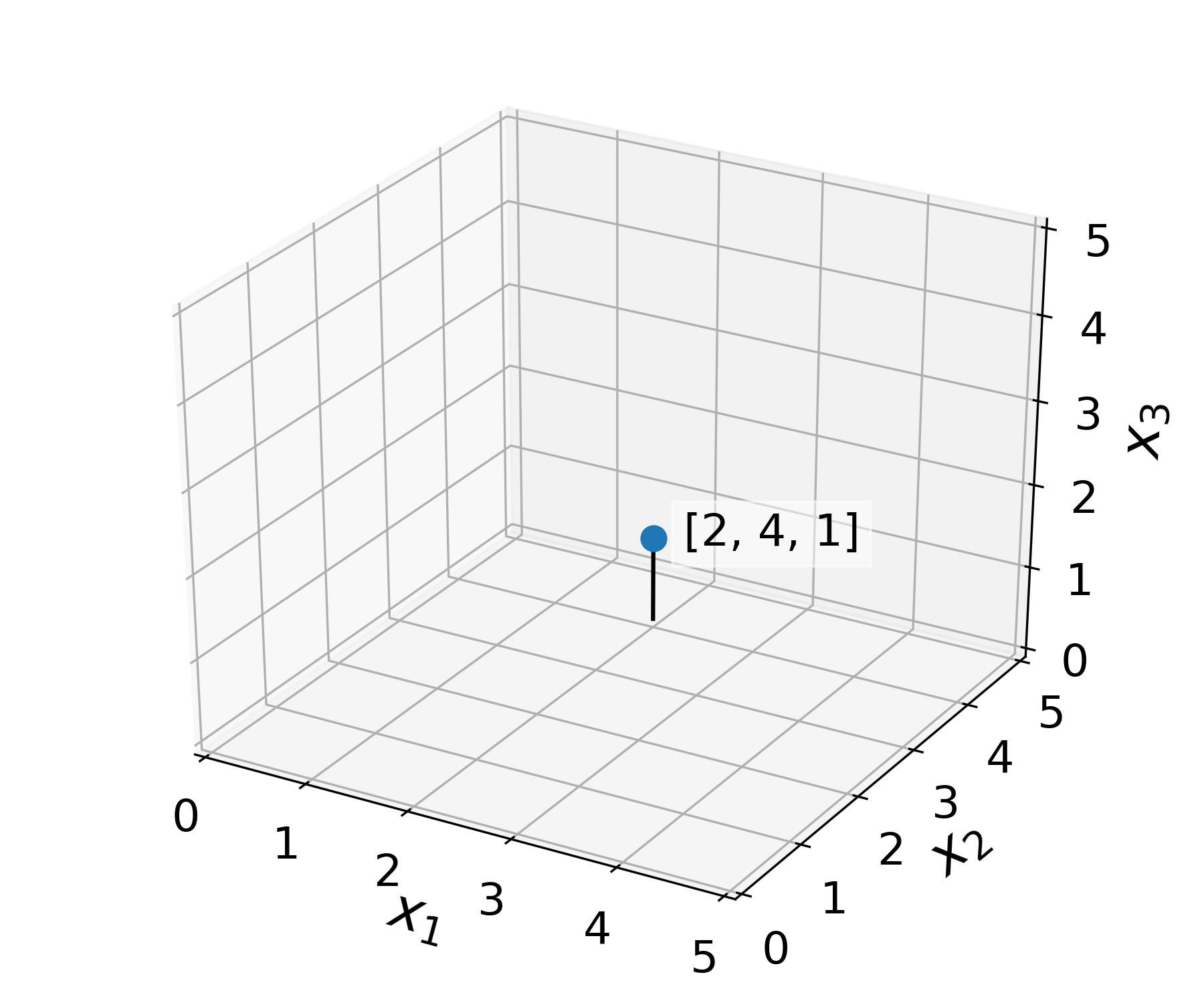
Here, the black line is simply there to help orient you to where this new point $\mathbf{a}$ exists in three dimensions. The point of this exercise is to get you understand how easily we can go from a space like $\mathbb{R}^2$ to something higher dimensional like $\mathbb{R}^3$. The difference between these two real coordinate spaces is not so scary. It’s the difference between a point drawn on a piece of paper and a point in the three-dimensional world in which we live.
A step up the dimensional ladder
At this point, I hope you feel comfortable with the concept of a vector in either $\mathbb{R}^2$ or $\mathbb{R}^3$. Now, what about the promised land of $\mathbb{R}^m$?
Defining an $m$-dimensional vector is easy.
$$\mathbf{a_m} = \begin{bmatrix}x_1\\x_2\\\vdots\\x_m\end{bmatrix}$$
But how do we look at our creation? This question is not so each to answer. The matplotlib package has handy plotting functions for 2-d or 3-d space. Hard pressed, we could add color to each point to visualize a fourth dimension and change the size of each marker ($\bullet$) to add a fifth. However, not only are these solutions will create a plot that’s hard to interprate. Even worse, there’s no way we to extend such tweaks to get us up to the realm of $\mathbb{R}^{20000}$ to $\mathbb{R}^{30000}$, which is where most genomes reside.
Unfortunately, we will need to address the problem of visualizing high dimensional spaces in a later section of this course. For now, I hope the idea of a point existing in an arbitrarily high-dimensional coordinate space is no longer foreign to you.
Enter the matrix

Now that you (hopefully) understand the concept of an $n$ dimensional vector, let’s start thinking about matrices. Matrices are like vectors, in that they are a collection of numbers. Generally, a matrix looks like this:
$$A = \begin{bmatrix} x_{1,1} & x_{1,2} & \dots & x_{1,m} \\ x_{2,1} & \ddots & & \vdots \\ \vdots & & \ddots & \vdots \\ x_{n,1} & \dots & \dots & x_{n,m} \end{bmatrix}$$
So now, what exactly is $A$? Unfortunately, this is not a straightforward question to answer. Matrcies can represent different kinds of things depending on the context. The best way to think about a matrix is that is is a contain for numbers that is indexed by rows and columns.
Right now, we’re going to focus on the data matrix, which is a collection of vectors of the same dimensionality. Typically, each row of a data matrix represents a vector and each column represents a dimension.
Let’s take a data matrix of 3 three vectors in $\mathbb{R}^2$.
$$B = \begin{bmatrix} 1 & 2 \\ 2 & 4 \\ 3 & 1\end{bmatrix}$$
The first column of $B$ holds all the values for each vector in $x_1$ and the second column holds all of the values for each vector in $x_2$. The first row represents the first vector that $B$ is holding, and we could access this vector by retrieving $x_{1,1}$ and $x_{1,2}$ from $B$.
Now, let’s introduce an important property of a matrix, it’s shape. The shape of a matrix is the number of rows and columns in the matrix. The shape of our arbitrary matrix $A$ is $(n,m)$. The shape of our data matrix $B$ is $(3,2)$. In numpy you can get the shape of an ndarray with ndarray.shape. Not too difficult!
To look more closely at $B$, let’s use our tools in Python to visualize our new matrix.
B = np.array([[1,2],
              [2,4],
              [3,1]])


fig, ax = plt.subplots(1, figsize=(5,5))

# A[:,0] returns the first column of A
# and A[:,1] returns the second
ax.scatter(B[:,0], B[:,1])

ax.set_xlim(xlim)
ax.set_ylim(ylim)

ax.set_xticks(np.arange(0, xlim[1] + 1))
ax.set_yticks(np.arange(0, ylim[1] + 1))

ax.text(1.1,1.7, '[1,2]')
ax.text(2.1,3.7, '[2,4]')
ax.text(3.1,0.7, '[4,2]')

fig.tight_layout()
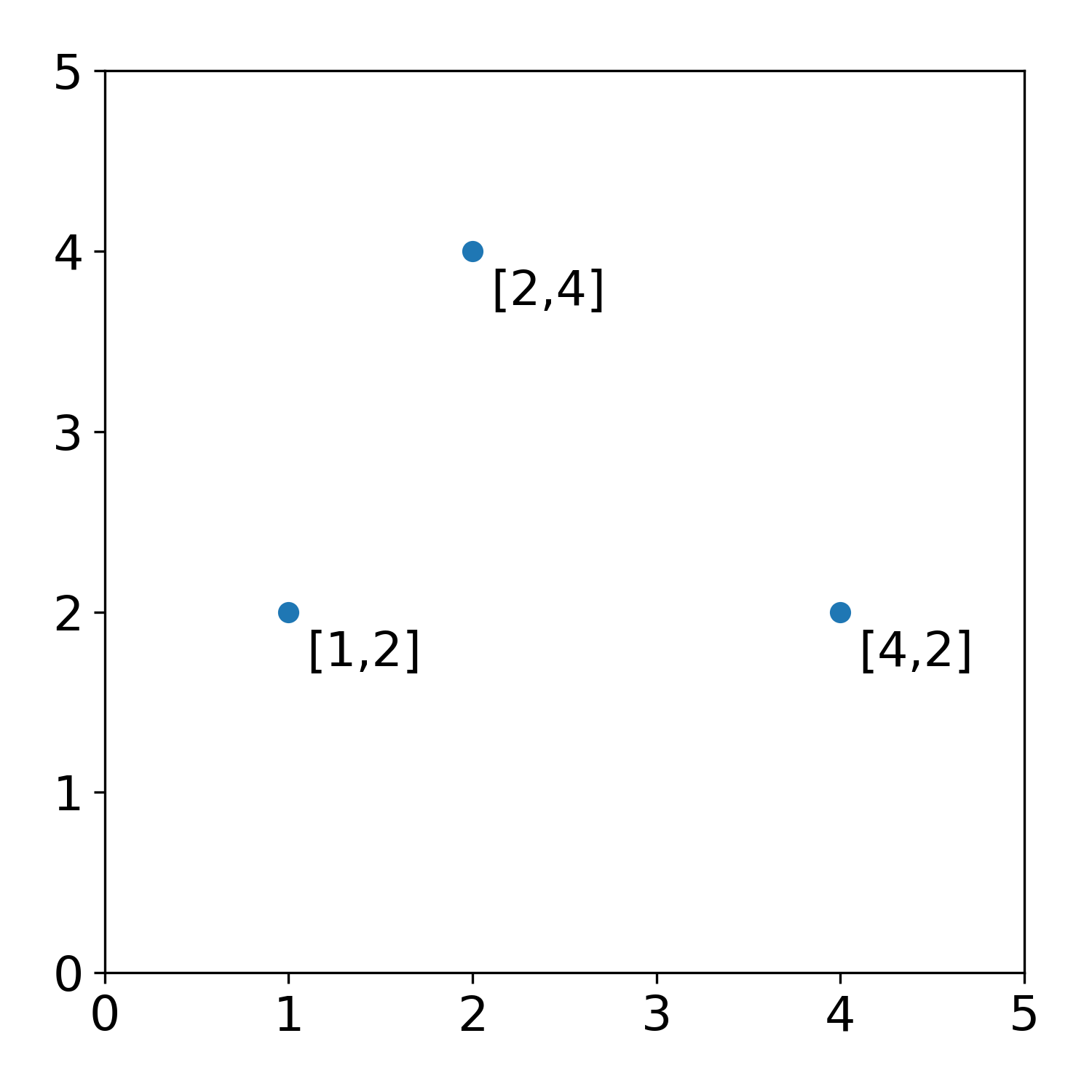
Hopefully it’s clear that adding a column to $A$ we could get a set of points in 3- or 4- dimensional space. The counts matrices we’re going to look at later are just an even higher dimensional extension of the simple data matrix $B$.
Now I said that there are other kinds of matrices besides the data matrix. One important one is the distance matrix, often denoted $D$. $D$ holds all of the pairwise distances between a set of points (i.e. vectors) in a given data matrix. To understand how we can create $D$ from $A$, we need to spend some time thinking about distance functions.
How far is it to there from here?
One of the most fundamental functions in data analysis is the distance function. A distance function $d(\mathbf{a},\mathbf{b})$ defines the distance between the two vectors $\mathbf{a}$ and $\mathbf{b}$ defined in $\mathbb{R}^{m}$. There are many kinds of distance functions. You’re probably most familiar with the Euclidean distance function which is defined as:
$$ d_{euclidean}(\mathbf{a},\mathbf{b}) = \sqrt{(\mathbf{a}_1 - \mathbf{b}_1)^{2} +(\mathbf{a}_2 - \mathbf{b}_2)^{2} + \dots + (\mathbf{a}_m - \mathbf{b}_m)^{2}} $$
Here the distance is defined as the square root of the sum of square distances in each dimension of $\mathbf{a}$ and $\mathbf{b}$. This distance function is useful because it works for most of the distance we encounter is every day life. If you have two airplanes that are flying at different altitudes and positions, you could calculate their distance longitudinally, latitudinally, and altitudinally and take the root squared differences to calculate the distance between them. Well actually because the earth isn’t flat this would be a little off, but you can imagine the concept.
There are many other distance functions, however. Take, for instance, the Manhattan distance:
$$ d_{manhattan}(\mathbf{a},\mathbf{b}) =\mid\mathbf{a}_1 - \mathbf{b}_1\mid +\mid\mathbf{a}_2 - \mathbf{b}_2\mid + \dots + \mid\mathbf{a}_m - \mathbf{b}_m\mid $$
Here we’re simply adding the distance in each dimension without any squaring or squarerooting. This distance would be useful if you want to calculate the number of city blocks a taxi would need to travel between two street corners in Manhattan.
Now Euclidean and Manhattan distances are both valid distance functions, and the decision to pick one over another will have an impact on how far two point are calculated from each other. To understand this, consider the three points that we defined in $B$ above.
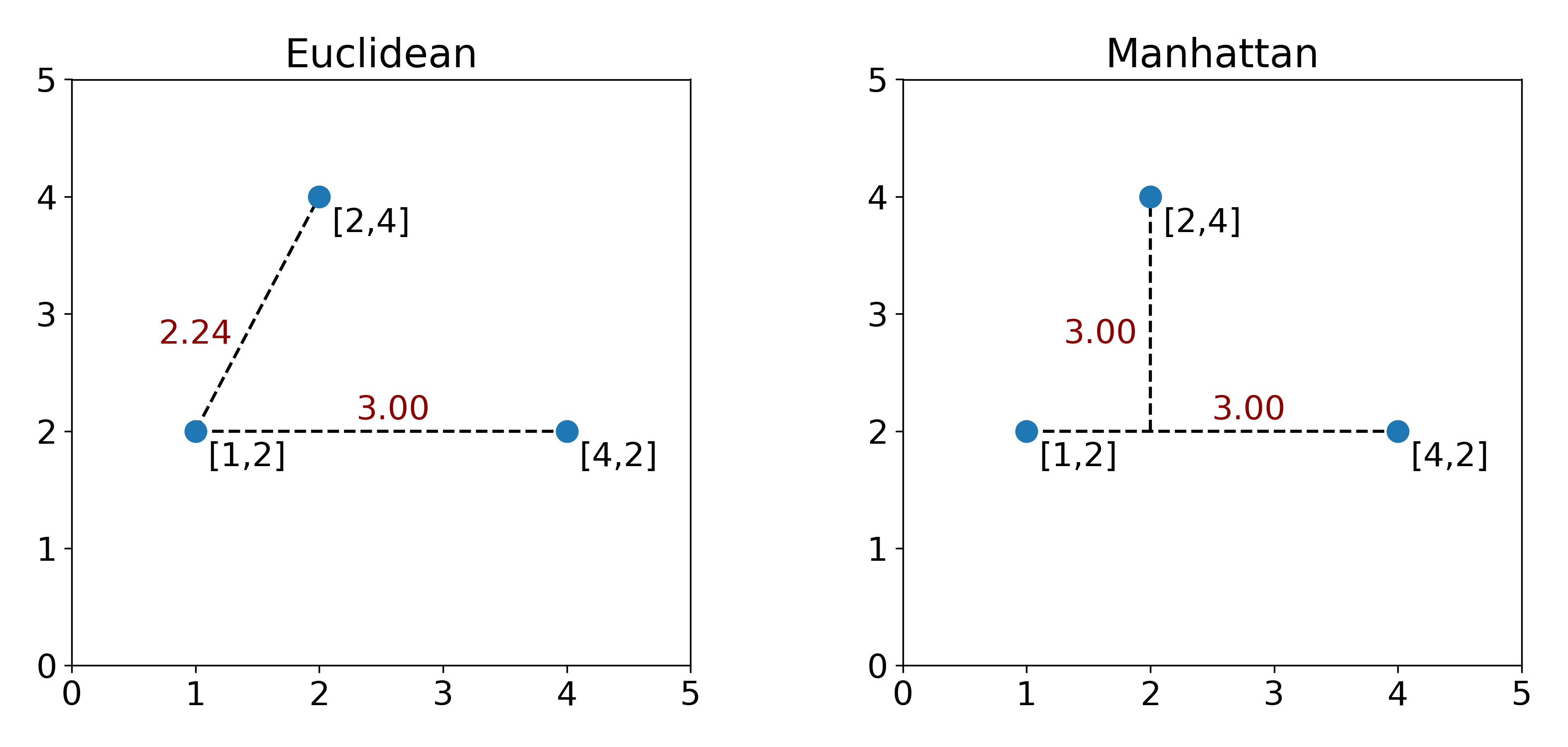
Now on the left and right plot, the points we’re looking at haven’t changed, but you can tell that the relative distances between points are different. At this point, we’re faced with a decision. Which distance is better? Math doesn’t have answer to this question, unfortunately. The answer will depend on what kind of data we’re storing in $B$. Are they cell counts? Are they street corner coordinates? For cells, we commonly use Euclidean distance, but is this the best possible distance function? Unfortunately there’s no easy answer here.
Representing distances in a matrix
Now that we have a handle on distances, we can create our first distance matrix. Let’s start by considering the Euclidean distance matrix from the points in $B$.
$$D = \begin{bmatrix} 0 & 2.24 & 3 \\ 2.23 & 0 & 2.82 \\ 3 & 2.82 & 0\end{bmatrix}$$
Unlike the matrices we’ve looked at before, $D$ is a square matrix. That means it has the same number of rows as columns. In a distance matrix, entry $D_{i,j}$ represents the distance from point $i$ to point $j$. You should notice here that the distances on the diagonal of $D$ are all 0, because one of the requirements of a distance function is that the distance from a point to itself must be zero. $D$ is also symmetric across the diagonal, another property of distances.
You can see looking up at the two plots above, that the entry $D_{1,2}$ is the distance between the first row ($B_{1,:}=[1,2]$) and the second row ($B_{2,:}=[2,4]$) of our data matrix. What a useful matrix to have!
Multiuse matrices
By this point, I hope you understand that matrices are powerful tools for representing properties of data. We’ve already encounter two important matrices. The first, the data matrix, can be used to store the raw data values associated with a set of observations. This matrix is like a data storage device. We can imagine adding rows or columns to this matrix just like and excel sheet as we collect more observations (rows) or pieces of information about each observation (columns).
On the other hand, the distance matrix stores information about a set of data. There are many data matrices that could produce the same distance matrix, but only one distance matrix per dataset per distance function. In this way you can this of a distance matrix as a descriptive matrix. Without any data, you have no distances.
As we will see in the next section, there are other useful kinds of descriptive matrices and ways of representing data and the relationships between points. One of the core models for data is the Graph.