What is single cell?

Recent advances in single cell proteomics and transcriptomics make it easier to collect single cell measurements across biological systems. Two of the most common methods are single cell RNA-sequencing (scRNA-seq) and CyTOF. Although we will focus on scRNA-seq in this tutorial, the concepts important for single cell analysis generally hold across technologies. This is especially true for visualization, clustering, and differential expression.

Why single cell?

Cells are one of the basic units of biology. We generally think of single cells as entities that act on themselves and surrounding extracellular structures to perform basic tasks such as moving appendages, processing external stimuli, defending the organism from infectious invaders, etc.. Because these units are so important for the functioning of an organism, it’s naturally to wonder how many different kinds of cells there are in a specific tissue, how these cells change over time, and how cells differ between individuals.

Although the genome provides information about all these phenomena, it is the differences in expression of individual genes (at the RNA and protein levels) that account for differences in function across cells. Because genes in individual cells effect functions in biological systems, measuring average expression across many cell types ,mixed at unknown ratios–as done in bulk RNA-seq–limits biological insight.

A brief history of scRNA-seq

Gene expression has been measured in single cells since at least 1992, when J. Eberwine et al. published the first single cell qPCR assay in Analysis of gene expression in single live neurons (1992). They measured expression of roughly one dozen genes in 15 neurons isolated from the brain of a rat and characterized two distinct populations based on ion channel expression. Shortly thereafter in 1998, developments in smFISH (single molecule Fluorescence In Situ Hybridization) provided the a way to visualize expression of individual mRNA molecules in single cells (Femino AM, et al. 1998). smFISH remains the current gold standard for single cell RNA quantification and is used for validation of many scRNA-seq methods. In 2003, Kamme F et al. expanded the set of genes assayable in single cells using microarrays (Kamme F. et al. 2003). In that study, a groundbreaking ~4500 genes were assayed in 11 cells.

All of the above methods rely on some method of hybridization to nucleic acid probes (i.e., they bind to a predetermined RNA sequence). It wasn’t until 2009, however, when RNA sequencing expanded single cell RNA profiling to the entire transcriptome (Tang, F. et al. 2009). This protocol and subsequent single cell protocols require the manual isolation of individual cells into PCR tubes for cDNA amplification. The time-consuming nature of this technique and high cost of preparing relatively large microliter-scale reverse transcription reactions kept dataset sizes down in the range of dozens of cells per sample. In 2012, Fluidigm introduced the C1 microfluidic device that (at the time) automatically captured up to 96 cells from a single cell suspension created single-cell libraries using nanoliter reaction volumes.

The biggest disruption in single cell transcriptomics arrived in the summer of 2015 when two groups at Harvard published independent microfluidics technologies to capture cells in nanoliter droplets (Macosko EZ. et al. 2015; Klein, AM. et al. 2015). The speed, scalability, and low cost of these methods suddenly made it possible to profile tens of thousands of cells in a single experiment. These droplet-based single cell approaches were commercialized by 10X Genomics in 2016 in their $125k lunch-box sized Chromium device (Zheng, GZ. et al. 2017). Since then, there have been several advances in single cell transcriptomics, including the ability to simultaneously capture cell surface epitopes and transcriptomes in single cells (Stoeckius M., et al. 2017) and efficient split-pool library preparation methods (Gierahn TM. et al. 2017). However, most of the data our lab analyzes comes from the 10X Genomics 3’ Single Cell library prep kit.

How to capture cells in droplets

Capturing mRNA from individual cells is a challenging goal. The first challenge is isolating individual cells for reverse transcription. In droplet based methods this is done using a microfluidic chip. The following schematic from Zheng, GZ. et al. (2017) shows how this works.

The chip captures beads loaded with barcoded library adapters and individual cells into droplets. These droplets form an emulsion because they are suspended in oil. In the next image, you can see a single looped cell capture event on a DropSeq chip.

Here, a single cell (bottom) joins a bead in lysis buffer (left) as they flow through the chip. Oil flows in through the channels in the middle and pinch off individual droplets.

Although the exact nature of the bead varies between technologies, the basic idea is that each bead contains uniquely-barcoded adapters with: an oligo d(T) that hybridizes to poly-A tails (one end of an mRNA transcript), a cell barcode, a unique molecular identifier, and reverse transcription primers.

scRNA-seq library preparation

Although you probably know this, let’s start by reviewing the basic structure of an mRNA.

In the standard 3’ library preparation, the goal is to select for mRNA using the polyA tail. Selection is necessary because the majority of RNA in a cell consists of ribosomal RNA (rRNA) and transfer RNA (tRNA). We don’t want to sequence these functional RNAs because they don’t give us information about gene expression. To select poly-adenylated mRNA, the library adapters include a long stretch of thymines (Ts) that hybridize with the long stretch of adenines (As) in the polyA tail.

La Manno, G. et al. (2018) found that these library adapters also prime internally (i.e. more 5’ than the polyA) making it possible to sequence the introns of newly-transcribed pre-mRNA molecules facilitating the detection of actively expressed genes.

Following hybridization of adapters, the basic steps for library preparation are as follows:

1. cell capture into droplet
2. cell lysis within droplet
3. 3’ barcoded-adapter hybridization to polyA tail of mRNA
   
4. first strand reverse transcription (RT)
5. second strand RT occurs
6. PCR amplification
7. fractionation and size selection
8. 5’ adapter ligation
9. final amplification
10. sequencing

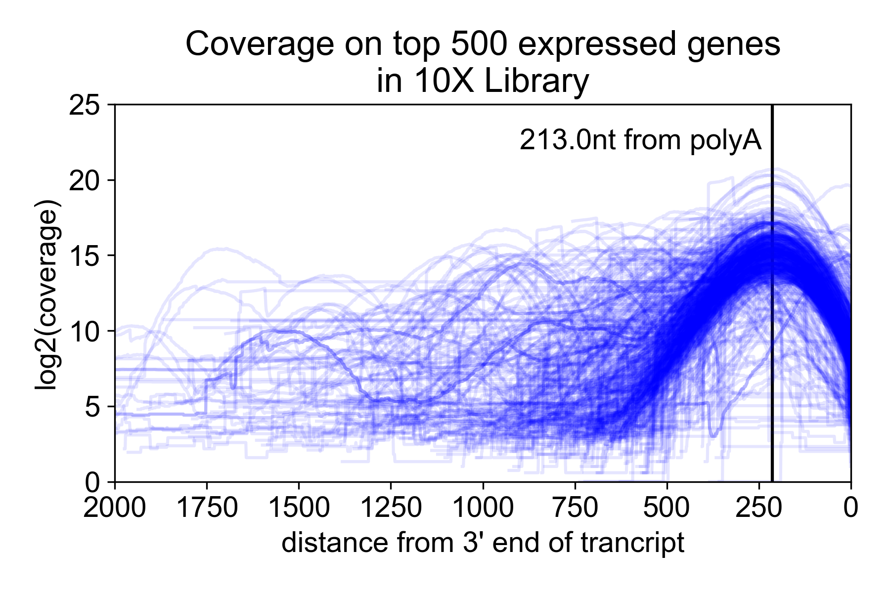
Because of the size selection and PCR amplification primed using the 3’ and 5’ adapters, the library is heavily 3’ biased with the majority of the read coverage falling ~200nt from the 3’ untranslated region (UTR) of the mRNA. Note, however, that annotated 3’ UTRs do not always correspond to the actual isoform expressed in a sample. For this reason, you may get coverage “past” the end of the gene.

In the following plot, I took the 9K PBMC dataset from 10X Genomics and plotted coverage over the top 500 expressed genes relative to the annotated 3’ UTR.

Special considerations for single cell data

Single cell datasets are unlike most other biological datasets for several reasons. First, these datasets are large. When analyzing bulk RNA-seq data, it is common to have roughly 2 to 10 datasets. A massive dataset, like the one generated by the GTEx (Genotype-Tissue Expression) consortium, might have 50,000 gene expression measurements. Compare this to the 1.3 million cells dataset generated by 10X Genomics in 2017. Even a lab with no experience generating large biomedical data can use scRNA-seq to measure gene expression in several thousand cells. The sheer number of observations in these datasets necessitate special computational approaches to analyze them.

Another reason that single cell datasets are challenging to analyze is they are high dimensional. Compared to more common single cell methods like FACS or single cell qPCR or microarrays, scRNA-seq datasets comprise many more features per cell. This makes it difficult to understand things like “which cells are close to which?” or “what genes are most similar?”. Thankfully, we can make some simplifying assumptions that make tackling these questions easier.

Because the data is high dimensional, it also makes inspecting the data challenging. How do you visualize the relationships between the cells or genes in your dataset so that you can identify cell types? We address this problem in our section on visualization.

Single cell data is also noisy. In scRNA-seq, it is estimated that only 10-40% of the hundreds of thousands of genes in a cell are captured during reverse transcription. Because of this, all genes in the cell are undersampled, and some lowly expressed genes might not get detected at all despite being expressed. Unfortunately, many of the marker genes we might be interested in are lowly expressed. This makes it hard to characterize cell types. Furthermore, this noise makes learning interactions between genes challenging. We discuss this problem in our section on imputation.

Single cell data is also prone to batch effects. Although easy to intuitively grasp, formalizing a definition of a batch effect for scRNA-seq is challenging. I think the most accurate definition of what we mean when we say batch effect is “variation present between datasets measured in separate batches that is 1) associated with having processed samples in separate batches and 2) not associated with relevant biological variation under investigation.” Now that’s very wordy, but I’m not sure how it can be precisely described with fewer words. What makes characterizing and normalizing batch effects challenging in scRNA-seq data is the second condition above. Simply normalizing two or more datasets so that there’s no difference between them is trivial. What’s difficult is disentangling trivial variations in gene expression from important ones. I think characterizing a batch effect is tied tightly to a specific question (one research might not care about variation in ribosomal proteins while another think they’re crucial). This is a very complex issue, and we’ll go into more detail in our section on batch correction.

Finally, more and more commonly researchers are preparing multiple single cell datasets and with the goal of characterizing the differences in cell states and gene expression between them. Quantifying such differences is challenged by biological and technical variation, incomplete experimental penetrance, and small effect sizes. As such, identifying the differences between single cell conditions requires specialized approaches. We’ll go into depth on this topic in our section on quantifying the effects of experimental perturbations.

Common goals for analysis of scRNA-seq data

With the above considerations in mind, it will be useful to consider what common goals of analysis you should think about as you sit down with any single cell dataset. This list is by no means exhaustive, but is meant to communicate potential avenues for analysis.

1. Cell type identification
   • How many kinds of cells are in the dataset?
   • What genes are differentially expressed between them?
   • What marker genes can be used experimentally to isolate each population?
   • Do there exist previously unidentified subtypes of cells?
2. Pseudotime analysis
   • What developmental trajectories exist in the data?
   • What genes change along those trajectories?
   • What is the ordering of cell states during development?
3. Gene-gene interactions
   • What genes are strongly associated with each other (i.e. co-expressed)?
   • What genes are potentially upstream of others?
   • How do these relationships change between cells?
   • How do these relationships change across time?
4. Comparing experimental conditions
   • What cell types change the most/least between conditions?
   • What genes change the most/least between conditions?
   • Which condition has the strongest/weakest effect on the underlying system?
   • Which conditions are most/least similar in their effect?

With these potential goals in mind, let’s get started with the first step in single cell analysis: Preprocessing!